We saw in Section 4.2 that in the real world, it’s more common to have data that is approximately linear than it is to have data that is exactly linear. The same thing is true of exponential models! Today, we will put the skills we’ve been learning together to analyze data sets with exponential trends.
A consequence of the relationship between \(\log_b\) and raising \(b\) to powers is that if we have data with an exponential trend and take the log of one of the variables, we get a new data set with a linear trend. Linear trends are easier to work with than exponential trends, so scientists use this trick to help them study data with an exponential trend.
Chart made in Excel using data from: Hannah Ritchie, Lucas Rodés-Guirao, Edouard Mathieu, Marcel Gerber, Esteban Ortiz-Ospina, Joe Hasell and Max Roser (2023) - "Population Growth" Published online at OurWorldInData.org. Retrieved from: https://ourworldindata.org/population-growth [Online Resource]
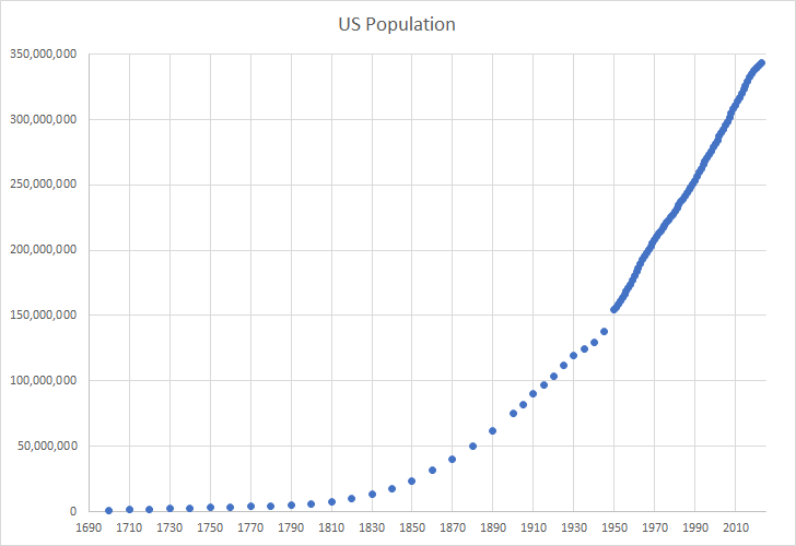
shows the population of what is now the United States between 1700 and 2023.
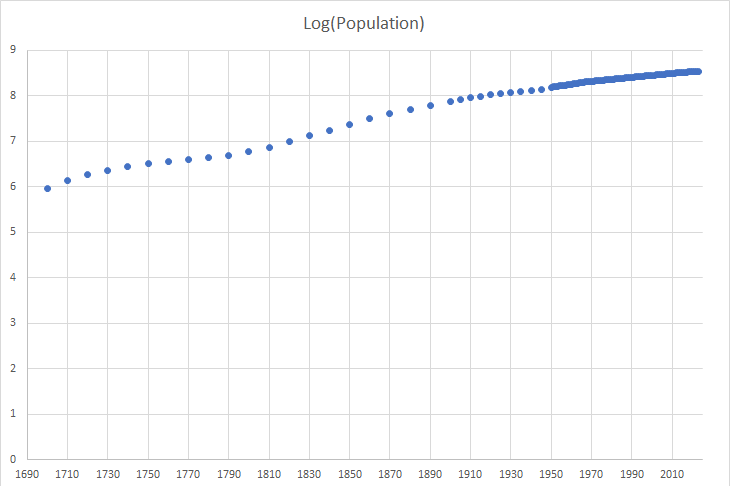
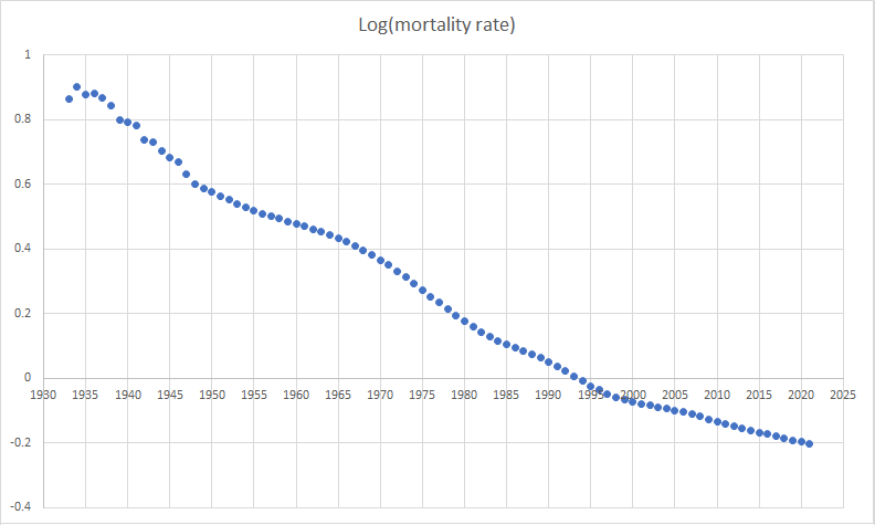
The trend of the population data resembles the graphs of an increasing exponential model. Logs are often used to analyze trends when the data seems to grow exponentially. The graph above right shows the log of the population. The years are kept the same, but the vertical axis shows the log of the population instead of the population itself. A graph that takes the log of the data values on one of the two axes is called a semi-log graph.
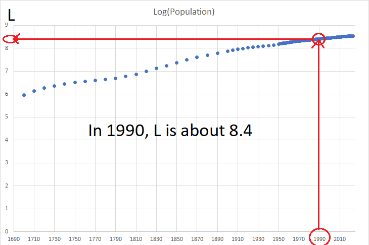
To estimate the output in 1990, go in a straight vertical line from 1990 on the horizontal axis to the curve. Then, go in a straight horizontal line from that point on the curve to the vertical axis. The value you hit on the vertical axis is the output. In 1990, the semi-log graph gives us an output of about 8.4.
We can use the value of \(L\) that we get from the semi-log graph to find the population. Since \(L = \log(P)\text{,}\) where \(P\) is the population, in 1990 we have:
\begin{align*}
L \amp \approx 8.4\\
\log(P) \amp \approx 8.4\\
10^{\log(P)} \amp \approx 10^{8.4}\\
P \amp \approx 251,\!188,\!643
\end{align*}
Use your value of \(t\) to find the year. (Depending on how you set up your linear model, \(t\) might already be the year, or you might need to adjust it.)
Fill in the last row of the table by taking the log of the cost values. Keep three decimal places! For example, in 1980, the value in the Log Cost row should be
Find a formula for a linear model for log costs. Use \(L\) as the output variable and \(t\) as the input variable, and include at least four decimal places in your slope.
Alia is an economist studying increases in prosperity in East Asia since World War II. One of the data sets that she’s using in her study gives GDP per capita between 1820 and 2020. 2
Table11.2.6.GDP Per Capita in East Asia, 1950 - 2020 (in constant international dollars at 2011 prices, to adjust for inflation and cost of living differences between countries)
Find a formula for a linear model for log GDP. Use \(L\) as the output variable and \(t\) as the input variable, and include at least four decimal places in your slope.
Sometimes it’s useful to undo the logs and get a formula for an exponential model for the original output variable. The key to doing this is to remember that
Let \(G\) be the GDP per capita and rewrite your formula by replacing \(L\) with \(\log(G)\text{.}\) Then, apply the “10 to the power of” operation to both sides of your equation to get a formula for \(G\text{.}\) Your formula should look like
\begin{equation*}
G = 10^{at + b}\text{.}
\end{equation*}
Use your formula for \(G\) to estimate GPD per capita in 2025 and to estimate when GDP per capita was $10,000. Do you get the same answers as you did with the linear model for \(L = \log(G)\text{?}\)
Graph each of the data sets given below, and use your graph to decide whether a linear model, an exponential model, or neither is a reasonable fit for the trend. If a linear or exponential model is a reasonable fit for the trend, find a formula for it.