We use “opposite” operations to solve equations. If you can see what operations are currently applied to a variable, you can do the opposite operations to solve the equation - to find out what number the variable stands for. Some examples of operations in math are: addition, subtraction, multiplication, division, raising a number to a power, and taking a root of a number (such as the square root).
Now, consider the following example. Even though both equations include the same numbers and the same variable, they are fundamentally different. It’s all about the placement of a variable.
An equation that has a variable in the exponent is called an exponential equation. Sometimes, we can solve such equations by inspection. This means we look at an equation and see what number could go in place of the variable to make the equation true, such as in the equation \(10^x=100\text{,}\)where we know that \(x = 2\) because \(10^2= 100\text{.}\)
Note: If a problem asks you to solve an equation by inspection, but you don’t have that arithmetic fact memorized and don’t see the answer, that’s okay! In that case, use the instruction to “solve by inspection” as a hint that the answer is probably a small nice number, and solve by guess and check instead.
In Section 8.1, we saw that we can also undo the operation in an exponential equation using logarithms, which are often referred to as logs. We learned to use the log operation to solve equations when the base is the number 10 (such as \(10^x=16\)).
You might be able to use inspection to see that the solution to \(7^x = 49\) is \(x = 2\) because you remember that \(7^2=49\text{,}\) but the answers to the other two examples are not nice numbers. To solve this problem, we have to tell our calculator to use a base other than 10 for our log. We write \(\log_b\) for the log base \(b\) operation. The log base \(b\) operation finds the exponent of \(b\) that gives us the number we’re looking for. For example,
But what numbers are \(\log_3(25)\) and \(\log_{1.05}(1.6)\text{?}\) Many calculators can only evaluate logs with base 10 or the special number \(e\text{.}\) To evaluate something like \(\log_3(25)\) using log base 10 instead of log base 3, we use that
The solution to \(1.05^x = 1.6\) is \(x = \log_{1.05}(1.6)\text{.}\) Turn this into a decimal using log base 10 and a calculator, then check your answer.
Solve each of the equations below. Write your answer in two ways: as \(\log_b(a)\) and as a decimal, rounded to the nearest thousandth. Double check your answers!
Suppose that the cost of attending a certain four-year private college (tuition and fees) was $16,500 in 1977 and that the cost increased about 3.2% every year.
\begin{equation*}
T = 16,\!500(1.032)^t
\end{equation*}
is a formula that models this situation where \(T\) is tuition and \(t\) is years since 1977. We then thought about how we might determine the year when tuition would reach $42,000. We considered various methods, such as guess-and-check (guessing different values and checking the results), to find a solution to the equation:
We also modeled the amount of caffeine Jacob has left in his body several hours after drinking a 16-oz coffee drink in Section 7.2. Suppose that Jacob has just consumed a 16-ounce cup of coffee containing 300 mg of caffeine.
If caffeine is being eliminated from Jacob’s body at a rate of 13% every hour, how long before three quarters of the caffeine has been eliminated? Enter your answer rounded to the nearest hour. (Hint: First, set up a model for the situation and then use it to answer the question.)
Exponential equations are often seen when working with accounts or loans that use compound interest. Compound interest occurs when interest is calculated on both the initial principal and any accumulated interest from previous periods. (Note: For comparison, recall that simple interest does not take into account the accumulated interest, that is, the interest each year is only based on the initial principal.) The equation for computing the amount of a loan, or in an account, that uses compound interest (assuming no change in principal) is
\begin{equation*}
A = P\left(1 + \frac{r}{n}\right)^{nt}
\end{equation*}
where
\(A\) represents the total amount of the loan or in the account.
Suppose that you take out a $2000 loan with a compound interest rate of 4%, compounded annually (once a year). If you make no payments, and interest compounds annually, in how many years will the loan balance double (reach or surpass $4000)? Think about this on your own for a minute before sharing your ideas in your group.
A log is an operation that combines two numbers to make a new number. The log operation combines the base and a target, and gives us back the exponent that we need to raise the base to to get the target. Just like when you learned the “raise to the power of” operation in a previous math class, practice is the key to feeling comfortable with this new operation.
In real applications, we nearly always use a calculator to evaluate logs. But, evaluating logs without a calculator is a useful practice drill when we’re first learning logs. This is uncomfortable at first, but it makes our brains think about what a log means and helps us to feel more comfortable using logs in the future. Don’t use a calculator for this activity, except to check your answer! The purpose of this activity isn’t to get the answers, but to practice thinking about how the log operation works.
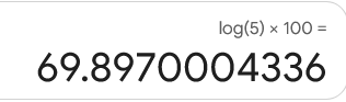
and he keeps getting it wrong. He doesn’t understand why - he’s entering it into Google’s calculator, so it HAS to be right. He presses the log button, then 5, then closes the parentheses, then times, then 100. Here’s a picture of his result:
Researchers often use logs to help them make charts when there are big size differences between the values in their data set. Alia is taking an astronomy class, and needs to make a chart showing the distance from the sun of the 8 planets.
Alia doesn’t like that the list of planets doesn’t include Pluto, so she decides to add it. She finds online that Pluto is 5925 million miles from the sun.